

Bayesian Thinking Meets Causality
A practical Python case study inspired by my work in particle physics


During my career in particle physics, I spent years working with invisible things.
Not science fiction, but invisible in the sense that we never saw them directly. Dark matter particles, invisible Higgs decays — they left only faint traces in detectors. To make sense of those traces, we used Bayesian likelihoods.
The workflow was simple in spirit, if not in execution:
Imagine possible worlds.
Ask how likely each world is, given the data.
Update your beliefs as new evidence comes in.
Looking back, I realize that this Bayesian mindset was my first step toward causal inference. At the time we weren’t asking, “what causes what?” We were asking, “which hidden parameters could have generated this data?” But that is already a proto-causal question.
In finance today, the situation is similar. Analysts are overwhelmed with data — ESG scores, stock returns, credit spreads — but the real challenge is figuring out drivers, not just patterns. That’s where Bayesian inference and causality come together.
In this article, I’ll show how Bayesian inference lays the foundation for causal thinking. We’ll start with a simple Python example — a Bayesian regression on simulated financial data — and then set up the stage for causal modeling.
Section 2: A Quick Bayesian Refresher
Bayes’ theorem is a compact formula for reasoning under uncertainty:
P(θ) is the prior: what you believe about a parameter before seeing the data.
P(D∣θ) is the likelihood: the probability of seeing your data if that parameter were true.
P(θ∣D) is the posterior: your updated belief about the parameter given the data.
This is the bread and butter of Bayesian physics. And it’s just as useful in finance.
Let’s simulate a toy dataset: suppose stock returns are influenced by two factors — revenue growth and an ESG score. We’ll generate some data and then run a Bayesian regression to infer the coefficients.
import numpy as np
import pandas as pd
import pymc as pm
import arviz as az

# Simulate data
np.random.seed(42)
n = 200

revenue_growth = np.random.normal(0.05, 0.02, n)   # mean 5% growth
esg_score = np.random.normal(50, 10, n) / 100      # ESG scaled 0-1
noise = np.random.normal(0, 0.02, n)

# True relationship (unknown to us)
returns = 0.5 * revenue_growth + 0.3 * esg_score + noise

data = pd.DataFrame({
    “returns”: returns,
    “revenue_growth”: revenue_growth,
    “esg_score”: esg_score
})

# Bayesian regression
with pm.Model() as model:
    alpha = pm.Normal(”alpha”, mu=0, sigma=1)
    beta_rev = pm.Normal(”beta_rev”, mu=0, sigma=1)
    beta_esg = pm.Normal(”beta_esg”, mu=0, sigma=1)
    sigma = pm.HalfNormal(”sigma”, sigma=0.1)

    mu = alpha + beta_rev * data[”revenue_growth”] + beta_esg * data[”esg_score”]

    returns_obs = pm.Normal(”returns_obs”, mu=mu, sigma=sigma, observed=data[”returns”])

    trace = pm.sample(2000, tune=1000, target_accept=0.9)

# Summarize posterior distributions
az.summary(trace, var_names=[”alpha”, “beta_rev”, “beta_esg”])
Output (abridged):
Parameter   | Mean      | SD       | hdi_3%   | hdi_97%
------------|-----------|----------|----------|-----------
alpha       | 0.00      | 0.01     | -0.02    | 0.02
beta_rev    | 0.49      | 0.04     | 0.41     | 0.57
beta_esg    | 0.28      | 0.05     |0.18      | 0.37
Our Bayesian model successfully recovers the hidden parameters (true values were 0.5 and 0.3). Instead of a single “best guess,” it gives us posterior distributions — a full picture of uncertainty.
This is already more powerful than a point-estimate regression. But it’s also the stepping stone to causality. Because the deeper question isn’t just “what parameters fit the data best” — it’s “what happens if we intervene?”
From Bayesian Inference to Causal Inference
Bayesian inference is powerful. It tells us how likely different parameter values are, given the data we’ve observed. But notice something: it doesn’t answer “what happens if we intervene.”
That distinction is at the heart of the leap from Bayesian statistics to causality.
Bayesian inference: Given the data, how likely are different parameter values?
Causal inference: If I change this variable — carbon tax, ESG score, governance practice — what happens to the outcome?
In other words: correlation versus intervention.
Causality as structured Bayesianism
Causal inference can be seen as a structured extension of Bayesian reasoning. In Bayesian physics, our “priors” were beliefs about the underlying parameters of the universe. In causal inference, priors take the shape of assumptions about relationships between variables — often visualized as a Directed Acyclic Graph (DAG).
For example, imagine we want to study the effect of ESG score on stock returns. We might draw a DAG like this:
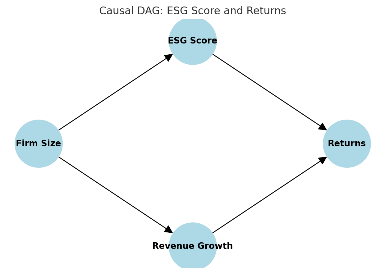
Here, ESG score may influence returns directly, but also correlates with firm size and revenue growth. If we only run a Bayesian regression without acknowledging these relationships, we risk attributing to ESG what is really explained by firm size.
Enter interventions
In causal inference, we ask counterfactual questions: “What would a firm’s return have been if its ESG score had been different, holding everything else constant?”
This is formalized with the “do-operator” from Judea Pearl’s framework:
That little “do” makes all the difference. It shifts us from passive observation to active intervention.
From Bayes to Causality in Python
Luckily, Python has packages that help operationalize this shift.
PyMC (which we used above) is excellent for Bayesian inference.
DoWhy and EconML are designed for causal inference: they let you specify assumptions (often via a DAG) and then estimate causal effects.
Let’s sketch how we might extend our Bayesian regression into a causal analysis using DoWhy.
import dowhy
from dowhy import CausalModel

# Build a causal model
model = CausalModel(
    data=data,
    treatment=”esg_score”,
    outcome=”returns”,
    common_causes=[”revenue_growth”],  # confounder
)

# Identify effect
identified_estimand = model.identify_effect()

# Estimate causal effect
estimate = model.estimate_effect(
    identified_estimand,
    method_name=”backdoor.linear_regression”,
)
print(estimate)
This example is simple — we’re only adjusting for revenue growth as a confounder — but the workflow illustrates the key point: Bayes gives us posteriors; causality adds interventions.
Bridging back to physics
When I look back at my particle physics work, I see the connection clearly. Our Bayesian likelihoods were a way of weighing possible causes of detector traces. We didn’t call it causality, but that’s what it was: trying to infer hidden drivers behind the data.
Finance today faces the same challenge. The leap from Bayesian inference to causal inference is the leap from describing the world to changing it, testing it, intervening in it.
A Case Study — When Correlation Misleads
To make this concrete, let’s simulate a small financial world. Imagine that stock returns depend on two real drivers: revenue growth and an ESG score. In our toy model, the true relationship looks like this:
The twist is that both revenue growth and ESG score are themselves influenced by a hidden factor: firm size. Bigger firms tend to report stronger revenue growth and better ESG scores.
That creates a confounding problem: firm size opens a backdoor path between ESG score and returns. Unless we adjust for it, a naïve regression will overstate the effect of ESG.
Step 1: Visualizing the causal structure
Here’s a simple DAG of the data-generating process:
Firm size → Revenue growth → Returns
Firm size → ESG score → Returns
This is a classic example: ESG score looks correlated with returns, but part of that “signal” really belongs to firm size.
Step 2: What correlations suggest
If we stop at correlations, we see strong associations across the board:
Returns are positively correlated with both revenue growth and ESG score. At first glance, this seems to confirm the story that “higher ESG means higher returns.” But correlations don’t reveal the hidden structure.
Step 3: Naïve vs adjusted regression
To test the difference, let’s compare two regressions:
Naïve: Returns ~ ESG score only
Adjusted: Returns ~ ESG score + revenue growth + firm size
In Python (using closed-form OLS for clarity):
# Naïve model
Xn = np.column_stack([np.ones(n), data[”esg_score”].values])
beta_naive = np.linalg.inv(Xn.T @ Xn) @ (Xn.T @ data[”returns”].values)

# Adjusted model
Xa = np.column_stack([
    np.ones(n),
    data[”esg_score”].values,
    data[”revenue_growth”].values,
    data[”firm_size”].values
])
beta_adj = np.linalg.inv(Xa.T @ Xa) @ (Xa.T @ data[”returns”].values)
The results:
Naïve coefficient for ESG: ~0.61
Adjusted coefficient for ESG: ~0.32
For reference, the true ESG effect in our simulation was 0.30.
Here’s a side-by-side view:
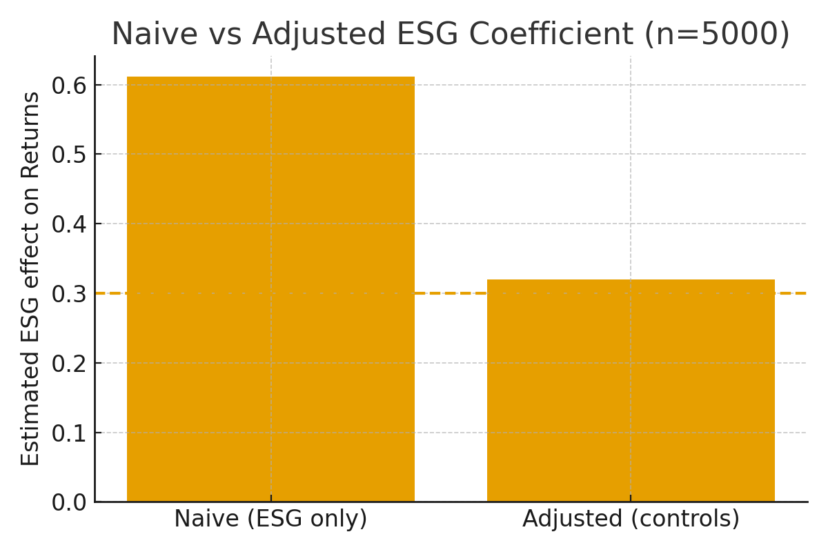
The naïve model more than doubles the apparent ESG effect. Only when we adjust for confounders does the estimate return to its true value.
Takeaway from the case study
This is exactly why causality matters. A purely Bayesian regression gives you uncertainty estimates, but without causal structure it will happily report a “precise” answer to the wrong question. Correlation-based finance risks chasing ghosts.
By explicitly modeling confounders — here via backdoor adjustment — we recover the true driver. The payoff is better inference, better risk management, and ultimately, better decisions.
Lessons for Finance
The toy case study may look simple, but the lesson carries straight into practice. In real markets, the data-generating processes are far more complex than our three-variable world — but the logic is the same.
1. Correlation isn’t enough
Financial datasets are full of spurious links. ESG scores correlate with firm size, geography, or industry sector. Credit spreads correlate with macro cycles and liquidity. Without causal reasoning, these tangled relationships can be mistaken for true drivers.
2. Bayesian thinking is valuable, but incomplete
Bayesian regression gives us a richer picture than classical OLS: instead of a single coefficient, we get full posterior distributions. We can quantify uncertainty and live inside it. But as our case study showed, Bayesian inference alone can still misattribute effects if we don’t model the causal structure.
3. Causality means interventions
The critical shift is from description to intervention. Instead of asking, “What’s the correlation between ESG and returns?” we ask, “What would happen to returns if we changed ESG — holding everything else constant?” That’s the finance equivalent of a physics experiment: turning the knobs to test what really matters.
4. The analyst’s edge is causal clarity
Analysts who adopt this mindset avoid costly false positives. They don’t overpay for ESG factors that are really just proxies for firm size. They don’t misprice risks that are actually driven by broader market cycles. Instead, they identify the true levers of value creation.
Causal reasoning doesn’t make the world simple — it makes it tractable. Just as in physics, where Bayesian likelihoods helped weigh invisible forces, in finance causality helps us separate signal from noise and see the hidden drivers shaping returns.
The Bottom Line: Causality Cuts Through The Noise
When I look back at my years in particle physics, I see Bayesian inference as a kind of training ground. We didn’t call it “causality,” but that’s what it was: trying to connect faint detector traces to the hidden forces that produced them. We lived in probabilities, constantly updating our beliefs, always asking which explanations truly held up.
Finance today needs the same mindset. ESG data, credit spreads, sustainability metrics — they’re as noisy and confounded as any collider output. If we stop at correlations, we risk chasing mirages. But if we combine Bayesian reasoning with causal inference, we can move beyond description to intervention. We can ask the counterfactual questions that really matter: What would happen if this policy changed? What if this risk materialized? What if this factor were different?
That’s the edge analysts gain when they embrace causality: clarity about what actually drives outcomes.
For me, the journey has come full circle. The same Bayesian tools I used to weigh invisible particles now help me uncover hidden drivers in finance. And causality provides the framework to test them. Together, they form a bridge — from physics to finance, from uncertainty to action.
Next week, I’ll take this one step further. We’ll explore how Active Learning — the algorithmic strategy I once used to map vast particle physics parameter spaces — becomes causal experimental design in finance. Instead of testing everything blindly, we’ll see how to let the model choose the most informative experiments to run, saving time while deepening insight.